by Steefan Contractor
(Find original post at Steefan’s blog, here).
I attended the ARCCSS/CLEX winter school from 25th-29th June 2018. The theme of the winter school was climate extremes and so it involved lectures in the morning on various climate extremes (such as heatwaves and rainfall extremes) and also a group activity in the afternoons. The groups were tasked with producing analysis investigating one of five complex questions which are listed below.
- Project A: Examine the influence of modes of climate variability on temperature extremes over Australia
- Project B: Examine the influence of modes of climate variability on precipitation extremes over Australia
- Project C: Examine the role of soil moisture preconditioning on the frequency and/or intensity of heatwaves
- Project D: Examine changes in drought and what this means for impacts in Australia
- Project E: Pick a recent extreme event. What are the natural and anthropogenic influences?
Each group was comprised of 6-7 students with various backgrounds and at various stages of their education. I think Melissa Hart, our ARCCSS/CLEX graduate director, did a great job allocating students to various projects that highlighted their skills as well as gave them an opportunity to improve in their weak areas. Since my PhD has focused heavily on observations, including the creation of a global dataset of daily precipitation, I have always felt like I could improve my climate model output analysis skills. As such I was very excited when I discovered that my group was allocated the fifth project, the detection and attribution project.
Right from the beginning I new what I wanted to get out of this project. I wanted to make sure that by the end of the project I new how to design and conduct an experiment that involves analysing climate model simulations. This meant knowing what the different model output variables are, what the various runs are (historical, future RCP projections, various forcings, various initial conditions etc.), what the various climate models are in ensembles like the CMIP5 ensemble, the structure and location of these variables on Raijin (Australia’s supercomputer), and where to find information on these variables.
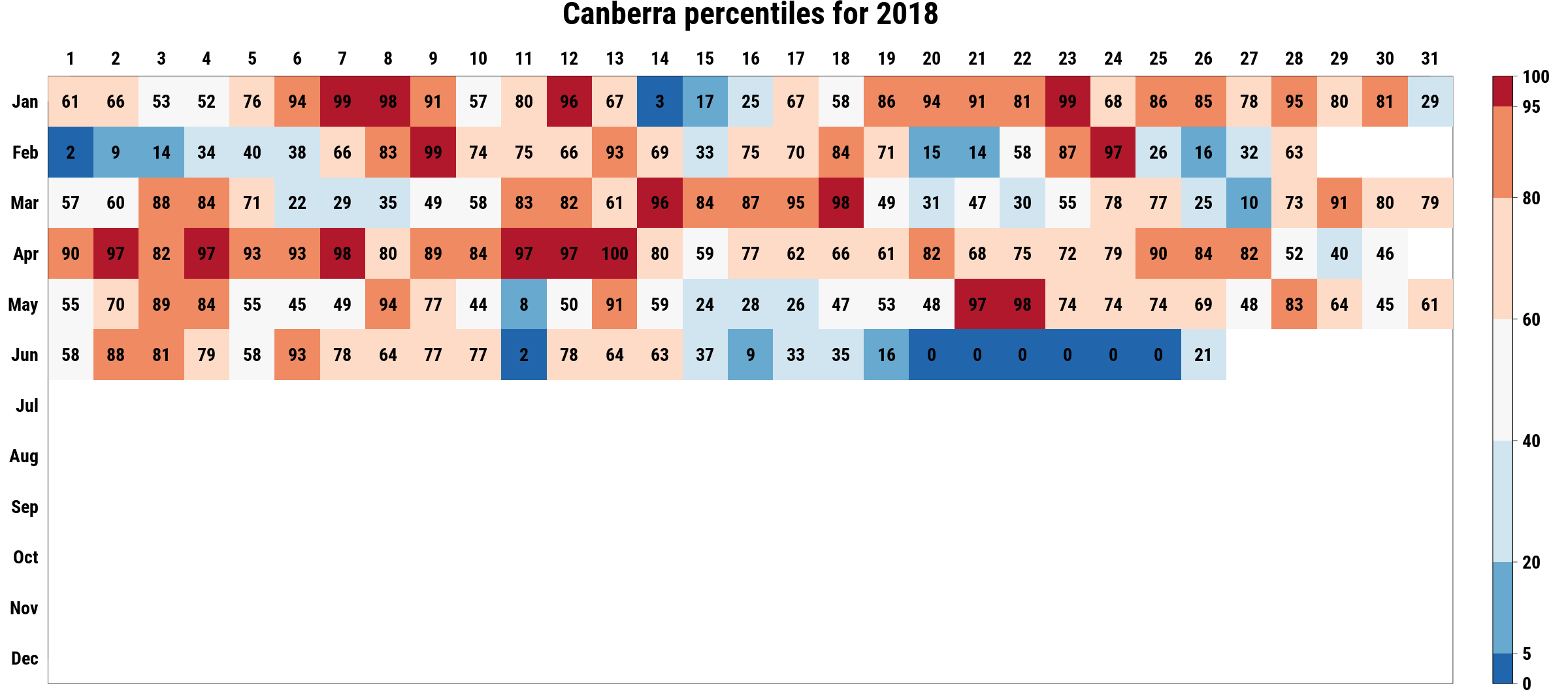
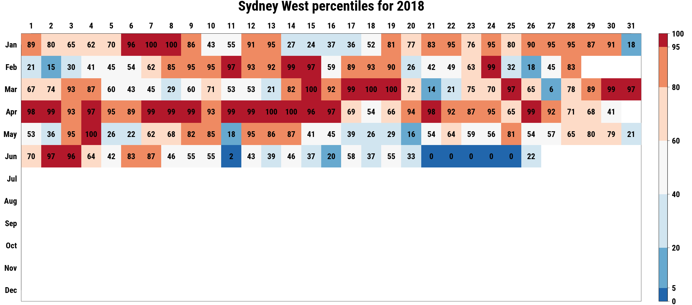
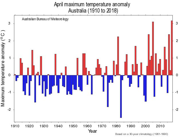
As a group we were keen to do event attribution on a recent event or at least an event that other researchers had not looked at yet. As a result we decided to look at the anomalously warm April we had this year. Based on the heatmap of temperature percentiles for 2018 on isithotrightnow.com, we were aware of the heatwaves in Sydney, Adelaide, Canberra and Alice springs in the middle of April. Upon checking the Bureau of Metoerology website, we discovered that 2018 April average Tmax temperature was hottest on record and 2018 April Tavg was second highest on record. Upon further research we discovered a conversation article which explained the conditions around the warmer than average temperatures in Australia at the time.
So why were temperature in Australia so high in April this year? The main reasons were the anomolously high Sea Surface Temperatures (SSTs) in the Tasman sea off the east coast of Australia which caused a low pressure off the east coast in turn weakening the cooling westerly winds, and the lower than average soil moisture conditions in Southern Australia at the time.
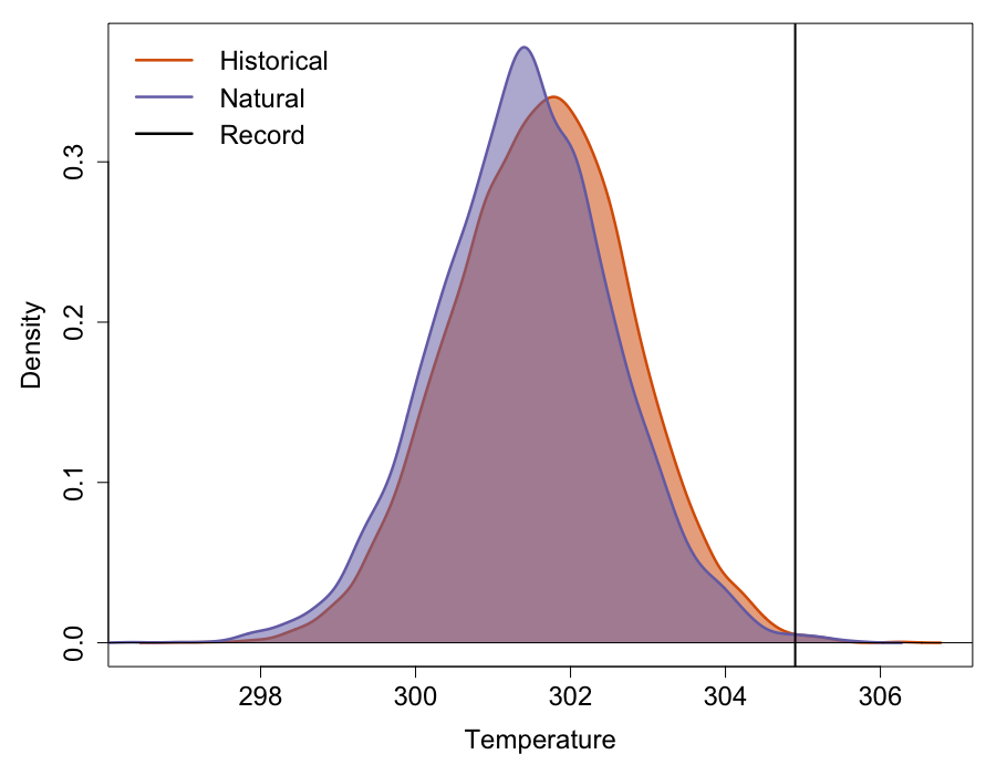
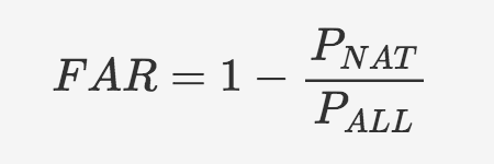
The experiment we decided to conduct was simple. The aim was to investigate whether the anomalously warm April Tmax average temperature was more likely in the current world compared to the natural world. We decided to look at the models in the CMIP5 ensemble to do this. There were 15 models on Raijin with both historical runs with all forcings, including anthropogenic (historical-ALL), and historical runs with only natural forcings, no anthropogenic (historical-NAT). The plan was to look at however many years of simulations in the various runs of each of these models and create a distribution of April average Tmax temperatures in historical-ALL runs and compare it with the distribution based on historical-NAT runs. We would then compute the fraction of attributable risk (FAR) value using the probabilities of April 2018 temperatures greater than or equal to our chosen absolute April threshold in these two scenarios (natural vs all-forcing).
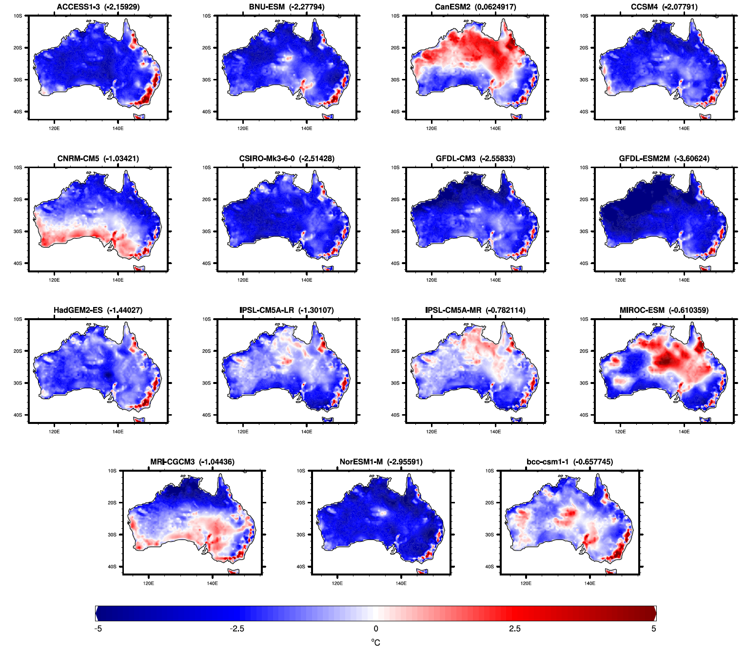
Since we are using an absolute threshold, however, we need to bias correct the models first. We did this by calculating the difference in means of April Tmax temperatures for Australia over 1961-1990 between historical-ALL runs of each model and observations, for which we used the AWAP dataset, and then added this difference back to the April 2018 Tmax temperatures for the respective models. Upon a quick discussion with Andrew King, I realised that bias correcting the models in this way assumes that the models are biased only in the means but not in the variance or skewness of the distribution. However, due to the time constraints of finishing the project during the winter school we decided to stick with our simple bias correction strategy. During our bias correction process, however, we realised that two of the models IPSL-CM5A-LR and IPSL-CM5A-MR were still biased. This could have been as a result of an error in the calculation of the bias or perhaps the bias in these models is not systematic in time, meaning the bias over 1961-1990 is not the same as the bias over the entire period of run for this model. In the end we decided to not use these models. The biases in our models are shown below, including the two models which we did not use.
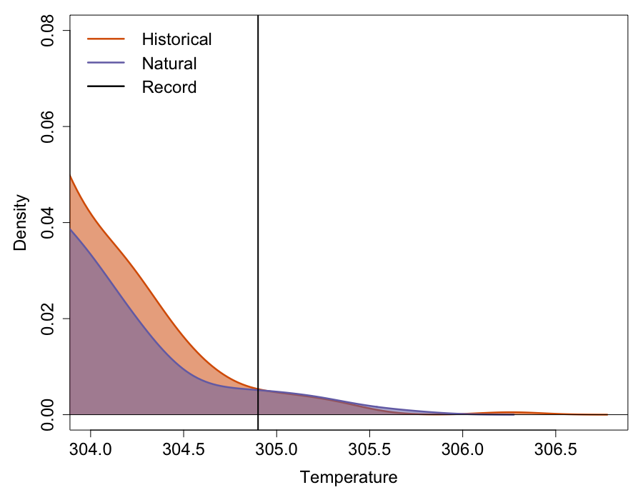
Our results (as seen in the main figure above the title) show that the historical-ALL distribution is shifted to the right compared to the historical-NAT distribution, however, the variance of the historical-ALL distribution is also smaller compared to the variance of the historical-NAT distribution. As a result, total area underneath the distribution to the right of the threshold (shown by the vertical black line) is actually smaller in the historical-ALL distribution compared to the historical-NAT distribution (as seen below). As a result, the resulting FAR value was -12.1%! During my conversation with Andrew King earlier, I was also informed that we can calculate the significance of our FAR value using bootstrapping. This is done by randomly sampling runs from both historical-ALL and historical-NAT runs and calculating the FAR value based on these. This process is repeated to create a distribution of our null hypothesis that the April 2018 Tmax temperatures are not more or less likely in the anthropogenic world. We can then test our FAR value against this distribution at a 10% level (5th and 95th percentile) to check for significance. We did not have time to conduct this bootstrapping exercise during the winter school but I suspect, had we done it, we would have found that our FAR value is not significant. My understanding is that the April 2018 event we chose is too extreme to accurately estimate the tails of the distributions because of the lack of estimates around the threshold. I believe if we chose a less extreme event we could have gotten a significant FAR value. The other possibility is that models cannot actually produce temperature this extreme given the initial conditions. Had we bias corrected the variance of the Tmax distributions for each model, we could have estimated the tails of the distribution better.
I think when it comes to event attribution, the actual FAR values should be given less emphasis anyway because of the uncertainties associated with the models and observations. I think we should be satisfied with statements that just say if the event in question is more or less likely in the anthropogenic world. Unfortunately we cannot with certainty make any such statements based on our analysis, although it looks like the event may not have an anthropogenic influence!
In terms of the future work related to this project, we clearly need to do the bias correction properly and also include an uncertainty based on the bootstrapping exercise. Based on the BOM data we also discovered that these anomalous April temperature were also the most widespread across Australia. So another interesting attribution exercise would be to attribute the spatial extent of this event to anthropogenic forcing. This can be done by once again choosing a local percentile based threshold for each grid cell to determine if the temperatures there are anomalous compared to the past. We can then count and compare the number of grids experiencing anomalous temperatures during April 2018 in the historical-ALL vs the historical-NAT simulations.
In summary, I thought the entire exercise served its main purpose which is that I now feel a lot more confident in designing and conducting experiments that involve CMIP5 model output analysis. A huge thanks to Melissa Hart, out ARCCSS/CLEX graduate director, for a great winter school!