… and figuring out which models simulate temperature extremes well for the right reasons.
Picture (above): Utah’s Green River flows south across the Tavaputs Plateau (top) before entering Desolation Canyon (centre). Credit: USGS (Unsplash).
Our ability to quantify future changes in regional daily temperature extremes relies on how well climate models simulate the main processes that explain historical extremes. Temperature extremes arise from many different physical processes, operating and possibly interacting with each other over a large range of temporal scales. These processes include the amplitude and persistence of cyclones and anticyclones, the influence of remote variability (e.g., El Nino Southern Oscillation), the background temperature and the response of the climate system to greenhouse gases and surface conditions such as the availability of moisture in the soil.
Climate models represent, in some form and with different levels of sophistication, the physical processes that are believed to play an important role in determining temperature extremes. However, what happens when a climate model represents one process accurately but represents another poorly? What happens when a model tends to exaggerate one process by, let’s say 2°C, while simultaneously underestimates another process by the same amount? The answer is that using traditional performance metrics, the model will appear to have a very small error because individual errors cancel each other out.
This issue of error compensation in climate models becomes more and more important as the climate phenomena being assessed increase in complexity and include more processes.
CLEX researchers addressed the error compensation issue for temperature extremes by defining a novel performance metric that identifies those models that can simulate temperature extremes well and simulate them well for the right reasons.
This was done by breaking up temperature extremes into four meaningful physical components:
- a long‐term mean annual cycle,
- a diurnal cycle,
- synoptic variability, and
- seasonal variability.
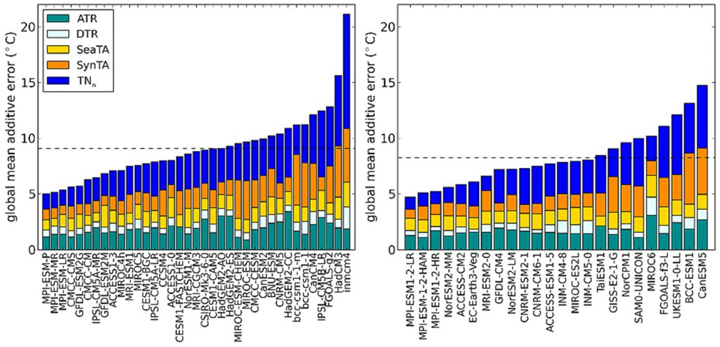
The researchers then calculated this decomposition for both cold and hot extremes as observed in multiple datasets and as simulated by 65 models from the Coupled Model Intercomparison Project (CMIP) Phases 5 and 6. The figure below shows the global mean “additive error” for individual CMIP5 (left) and CMIP6 (right) models. Models are ranked from lowest to highest additive error, and, for each model, the additive error is broken into the contribution from individual terms. Both panels show that the range of additive errors is very large with poor performance models having errors that are 3–4 times larger than best performers. Models with large additive errors usually show large contributions from the synoptic part of the extreme anomaly (SynTA) and from the cold night extreme (TNn) terms.
Figure: Full bars show global‐mean additive errors (full bar) for individual CMIP5 (left) and CMIP6 (right) models and the contribution to the total additive error by individual decomposition terms is shown using different colours. ATR is the annual temperature range, DTR the diurnal temperature range, SeaTA the seasonal temperature anomaly, SynTA the synoptic temperature anomaly and TNn the cold minimum temperature extreme.
Our results show that the overall performance of an ensemble improves when increasing the horizontal resolution largely due to improvements in synoptic scale variability. We also find that CMIP6 improvements relative to CMIP5 (about 10% on average) surpasses those expected from the increase in horizontal resolution alone suggesting that there have been model improvements associated with representation of physical processes.
Finally, our results highlight the reality that some current climate models can simulate global temperature extremes with considerable skill, and a low overall additive error. Determining what it is with these models – why they have so much more skill than some other models, provides a strategy to significantly reduce the overall ensemble error in future CMIP phases. Given we know it is possible to simulate climate extremes with a global mean additive error of about 5oC, one could set a benchmark for CMIP7 that to be included in the ensemble a model must meet a 5oC error benchmark. After all, the Max Planck Institute for Meteorology has demonstrated it is possible.
- Paper: Di Luca, A., Pitman, A. J., & de Elía, R. (2020). Decomposing temperature extremes errors in CMIP5 and CMIP6 models. Geophysical Research Letters, 47, e2020GL088031. https://doi.org/10.1029/2020GL088031

