What does climate model resolution mean?

Climate model resolution refers to the size and complexity of the data calculated by supercomputers to help us understand the weather and climate.

“Resolution” is a concept we see in our everyday lives but might not even realise.

Have you ever seen a picture on the internet and thought it looks blocky or fuzzy?

Computers break pictures down into small squares called “pixels”.

The more squares or pixels a computer uses, the more detail you can see in a picture, but if a computer uses fewer pixels it can load your picture faster. This is called the resolution.

Climate model resolution is similar, but on a much larger and more complicated scale.

A higher resolution climate model will have more information, but might be too expensive or take too much time to calculate.

A lower resolution climate model will have less information, but is easier and faster for computers to calculate.

What is temporal resolution?

Temporal resolution refers to how often climate variables are re-calculated, or the length of the time step used in models. Calculations are made for distinct blocks of time (often 20- or 30-minute blocks), which is called time stepping – for example 20- or 30-minute time steps are repeated until the desired length of simulation is completed. The length of timesteps and simulations can vary.

For example, measuring just a climate variable such as temperature, wind and humidity for every grid point every 30 minutes involves over 1.7-million-time steps in a century-long simulation! Doing the maths, 2 x 24 x 365 x 100 = 1700000!

What is spatial resolution?

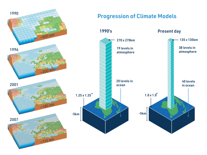
Spatial resolution refers to the size of grid cells in a model. Just as the temporal resolution determines how close in time to make the calculations, the grid size determines how close in location to make calculations. Climate model resolution, or the size of a grid cell in a climate model, is important.  A large or coarse resolution climate model grid square may represent an area of 200km by 200 km (40,000km²).

For example, for a single simulation of temperature provided for an area of 40,000 km² (similar in size to the state of Tasmania – land area 70,000kms), only two grid cells would be represented in such a model.

Smaller grid cells, or a finer resolution model, increase the spatial resolution, which can be as small as 2.2km by 2.2km ( approximately 5 km²) to around 50km by 50 km (2,500km²). This means more detailed information however it still only represents a single calculation for temperature, rainfall or wind for an area up to 2,500 km², which is roughly the size of the Australian Capital Territory.

Increasing the resolution of a climate model takes a lot more computing time. A rule of thumb is that doubling the resolution adds roughly a factor of 10 to the computing resources required. Climate simulations can often take 6 months to complete and increasing this to 60 months is impractical. In addition, increasing resolution can lead to vast amounts of data to manage. Both issues increase time and cost or could be too large to be run even on a supercomputer.

Example: Can we run a climate model at 5km instead of 10km?

Yes, but it would take a long time!

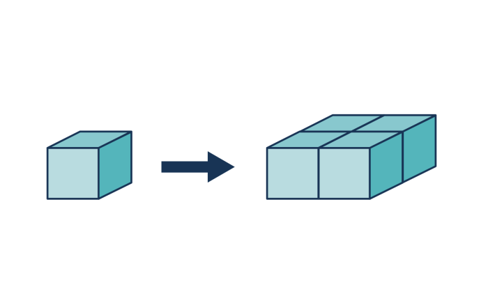
Climate models are 3-dimensional so if you double the resolution i.e., instead of looking at 10km square grid cells we look at 5km square grid cells, the number of grid squares increase to 4 grid squares to process instead of 1 . This is because you are doubling the  length and width.

For some models, resolution can be changed in the horizontal or vertical, rather than both, depending on the type of detail required.  

Does the grid size affect how we simulate climate processes?

Yes. Some processes will act on scales smaller than the grid cell size of the model. For example, a 50-km grid box excludes thunderstorms or patterns of vegetation which can be a few kilometres in size. Using a 1-km grid cell model will simulate the thunderstorm with more detail, however even this grid size may not contain small clouds which are indicative of thunderstorms.

Adding to this, some smaller processes are faster processes e.g., a thunderstorm which will evolve on a timescale of minutes.

Therefore, many smaller processes are represented in climate models using mathematical or simplified statistical approximations, called parameterisations.